
The Big Square with the Missing Corner
How the Sulbasutra approximation helps us derive a series expansion for √2

My book The Imperishable Seed: How Hindu Mathematics Changed the World and Why This History Was Erased, is available at
https://garudabooks.com/the-imperishable-seed
and
https://www.amazon.in/IMPERISHABLE-SEED-Mathematics-Changed-History/dp/B0BG7RRLVR


Abstract
A series expansion for the square root of two based on the sulbasutra approximation is derived. The first few terms of the series are given below:
The Sulbasutra Aprroximation for the Square Root of 2
A few years back I had visited the website of Professor David Henderson, late Professor of mathematics at Cornell University, where he had given a fascinating account of the method presumably used by the composers of the Sulbasutras in arriving at their highly accurate value for √2. Due to other priorities I could not read it in detail, so I bookmarked it for later reference. Later, when I did get the time, the website had been taken down by Cornell University. Slightly upset, I thought of reaching out directly to Professor Henderson, but a cursory search on the internet quickly yielded the sad news that he had already passed away in 2018.
This was disappointing, but a bit more hunting around revealed that he had published an article called Square Roots in the Sulbasutras in the volume Geometry at Work, a collection of articles edited by Catherine A. Gorini and published by the Mathematical Association of America in 2000, which promised to be the same as the one that had been taken down, at least as far as the content was concerned [1].
Some more searching, and I was able to locate a second hand copy of the volume selling on Amazon and shipping to Germany for the rather princely sum of 25 Euros. I clicked at the right places, and in a few weeks the volume was delivered to my place some time in July 2023, where again, what with the priorities of life taking over, it kept adorning my bookshelf, waiting till its time would come.

This finally came in April this year. Following a wonderful discussion I had had with Dr. Sai Priya of the Brhat Foundation on my book The Imperishable Seed: How Hindu Mathematics Changed the World and Why This History Was Erased, I was invited by Brhat to give a course on Hindu Mathematics on their platform. It was during the preparation of the course material that I finally sat down with the book and got myself to work through Henderson’s article, a considerable part of which I discussed in the course. However, what I did not discuss were the detailed mathematical steps and the derivation, as these would have been totally unsuitable for the course format. However, it is these details, and of course the writings of Bibhutibhushan Datta on which Henderson’s article is ultimately based, along with some other considerations, which showed me how so many rich and interesting ideas can be contained in a seemingly simple concept such as a square root, and so I thought it would be a good idea to discuss these along with some other interesting aspects in this post. Moreover, Henderson’s method along with many other finer aspects are not described in detail in most of the online resources on the Sulbasutras, so I thought this was one more good reason to write about this.
I will start directly with the sutra which gives an approximation for the square root of two. This is given in the Baudhayana Sulbasutra i.61 and i.62:
प्रमाणं तृतीयेन वर्धयेत्तच्च चतुर्थेनात्मचतुस्त्रिंशोनेन।
सविशेषः।
Translation: Increase the measure by its third and this third by its own fourth less the thirty-fourth part of that fourth. The name of this increased measure is savisheshah.
In today’s notation, the above sutra says that the root of 2 is given by the following approximation:
Moreover, the qualification savisheshah explicitly says that the result exceeds the actual value. In terms of usual fractions it turns out to be 577/408, whereas in decimal notation it turns out to be
which is correct to five decimal places.
Apart from its high accuracy, what is really interesting is the way the result is expressed, as it offers clues as to how it could have been derived. It is legitimate to ask, is there a reason it’s given like this, or is it simply coincidence? After all, they could simply have given it in terms of the final fraction, as was done on the Babylonian tablet YBC 7289 (for details see my earlier article). The first person who tried to offer an explanation for the above approximation after the publication of Thibaut’s translation of the Sulbasutras was Thibaut himself. In fact, in his 1875 article itself, where he translated parts of the Sulbasutras into English, and through which the Western world came into contact with the Sulbasutras for the first time, he attempted a reconstruction of the aforementioned Sulba approximation [2]. It goes as follows. According to Thibaut, the Sulba authors noticed that the area of a square with side of length 17 is 289, while the area of the square formed by the hypotenuse of an isosceles right angle triangle with side 12 equals, using Baudhayana’s sutra for the diagonal of a rectangle (“Pythagoras Theorem”, about which I’ve written here) 2×12²=288, which is quite close to 289. So, as a first approximation one can set 17²≈2×12², which gives √2 ≈17/12. This is actually an overestimate, since 17² exceeds 2×12². To obtain a better approximation, Thibaut proposed that the authors of the Sulbasutras again considered a square with side 17, and attempted to remove a strip of width x from two perpendicular sides, with x appropriately chosen, in such a way that the resulting square has an area of 288, i.e. 2×12². Then the length of the side of the new square is 17−x, and (17−x)²=288=2×12², so that √2 = (17−x)/2.
How should be x chosen? Thibaut’s hypothesis was that the Sulbasutra authors took away a strip of breadth x from one side of the square of length 17, so that the resulting area was 289−17x, and after taking away a strip of breadth x from an adjoining side, they took the resulting area to be 289−34x. Note that the two deductions result in the small corner square of side x (i.e. of area x²) being deducted twice, so that x² must be added to 289−34x, i.e. the actual value of the area of the new square should be 289−34x+x². But since x is smaller than 1 (if it was not, the new square would have an area lesser than 288, as can be verified), they, according to Thibaut, did not include the x² term. This is also sensible because otherwise they would have to solve a quadratic equation whose solution would involve √2, exactly what we are trying to find. So, after dropping the x² term and solving for x, we get 577/408, which is equal to the Sulba approximation.
Thibaut’s proposed reconstruction is possibly the simplest and the most intuitive possible. However, it suffers from a drawback, and that is, it does not explain why the Sulba approximation is given as a sum of four different unit fractions instead of stating 577/408 directly. As we will shall see below, there are natural reconstructions which yield the original Sulba expression. The first of these, and the one which is most generally accepted, was given by Bibhutibhushan Datta [3]. Apart from the fact that Datta’s method reproduces the exact Sulba expression, it has the major advantage that it has a direct connection with one of the sutras which offers a generic method for transforming a rectangle into a square. The sutra in question is Baudhayana i.54:
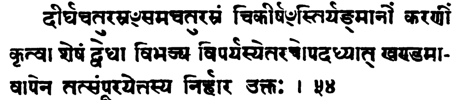
Translation (from Henderson): If you wish to turn a rectangle into a square, take the shorter side of the rectangle for the side of a square, divide the remainder into two parts and, inverting, join those two parts to two sides of the square.
Datta’s argument goes as follows. Take a rectangle with sides of length 2 and 1 and divide this into 2 equal squares of side 1 each (as shown in the left panel of the figure, where we have called A as the first square). Divide the second square into three equal rectangles as shown, (two of these rectangles are called B and C in the figure). The sides of these rectangles are one and one-third. Divide the third of these further into a square of side one-third, (shown by D in the figure), and divide the remaining into 8 equal smaller rectangles of sides one-third and one-twelfth, (named E to L in the figure).

Now rearrange the parts A, B, C, . . . J, K, L as shown in the panel on the right in the above figure. This results in a square with a small square of side 1/12 missing at the top right corner (this motif of a square with the missing corner will occur repeatedly, hence the title of this post). Ignoring the missing corner, the length of the side of the big square is 1+1/3+1/(3·4), which equals 17/12. Readers will notice that a part on top is missing so that the actual value of the square root of 2 is a bit less. In today’s terminology, we can call this reduced part by x and ((17/12) − x)² = 2. Expanding and ignoring the x² term gives the Sulba approximation 1+1/3+1/(3·4)-1/(3·4·34), which I’m mentioning here just for reference. This was not the method proposed by Datta. Datta’s proposed method relied on geometric rearrangements similar to the one. Let me walk through Datta’s method.
As mentioned, the the big square with the missing corner has a side of length 1+1/3+1/(3·4), i.e. 17/12. This is our initial approximation to √2, which we call L0:
The missing square on the top right has a side of length 1/(3·4) i.e. 1/12. We will attempt to fill this gap now by removing a strip of width w0 along the bottom horizontal and the left vertical sides such that the total area removed fits into the square gap on the top right, as shown in the following figure. w0 can be calculated as follows. The bottom horizontal and the left vertical both have lengths L0 = 17/12. Hence the area removed when the bottom strip is taken away is L0w0 = (17/12)×w0. The area removed when the left vertical is taken away would have been also (17/12)×w0, but for the fact that a square of side w0 at the bottom left corner is being removed twice. For the moment we ignore this and pretend that the area being removed is again (17/12)×w0. Hence the total area removed is twice this, that is, (34/12)×w0. This is set equal to (1/12²), the area of the missing corner at the top right. Solving for w0 gives w0 = 1/(34×12) = 1/(3×4×34):
where winitial = 1/12.
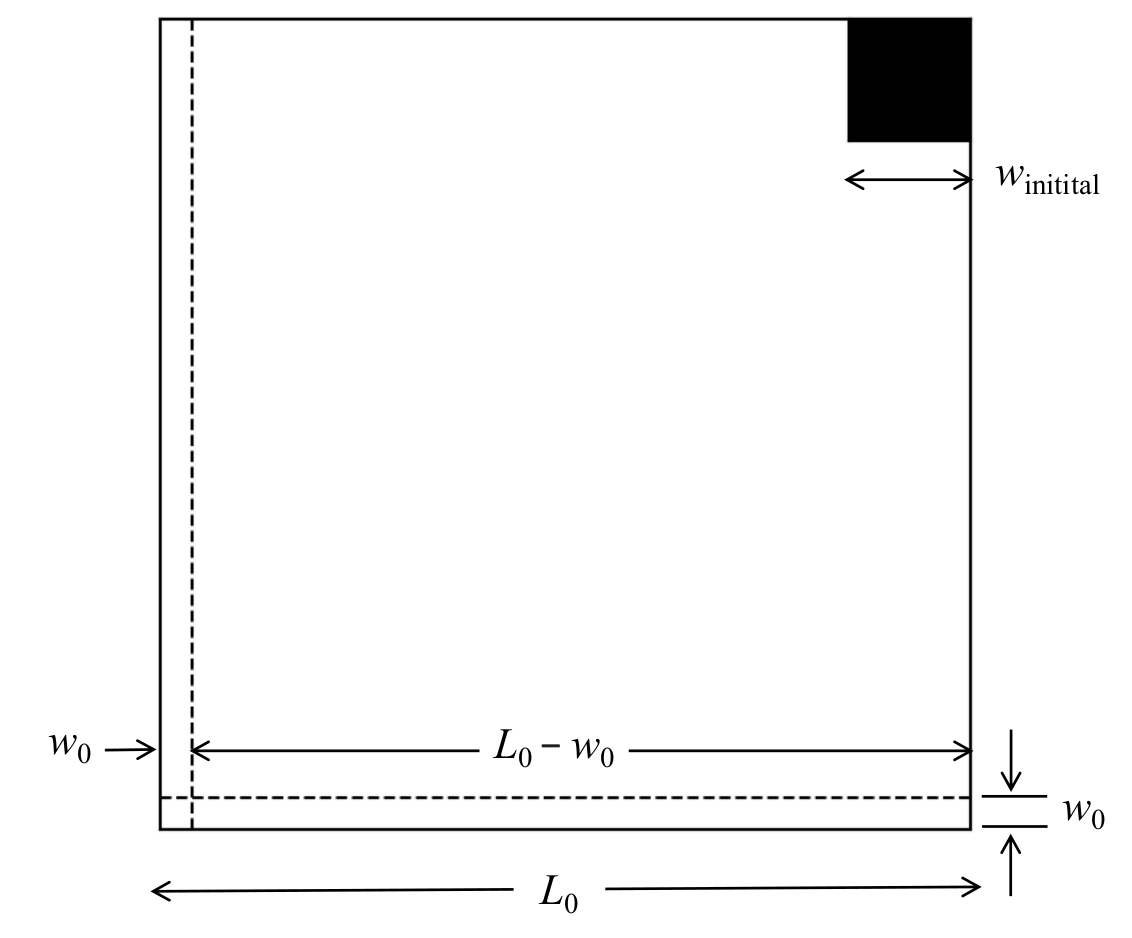
Note that area of the white region above equals 2, as this is simply a rearrangement of the rectangle with sides 2 and 1. The area of the black square is winitial², and the area of the big square is L0², Hence L0² = 2 + winitial².
The question remains: how to arrange the deducted strips into the top right corner? Note that the top corner has side of length 1/12, which we have called winitial. The strip from the bottom edge has length L0 = 17/12 i.e. (1+(1/3)+(1/3·4)). This has to be divided into smaller strips of length winitial to fit in the upper right corner square. How many strips should these be in total? This is given by L0/winitial = (17/12) ÷ (1/12) i.e. 17. Doing the same with the strip on the left gives us again 17, so 34 strips in total, which we can arrange in the missing corner on the upper right. These would have fit into the corner perfectly, but for the fact that we have removed the square of side w0 from the bottom left corner twice, whereas we can of course remove it only once. So the strips will not fit perfectly into the corner; rather, a gap of area w0² will still remain after the strips have been fitted. We can place this gap as a square of side w0 at the top right corner.
Once the rearrangement is made, the new length of the side of the big square will be lesser by an amount w0 than the earlier length of L0, which is our next approximation to √2. We call this L1:
This is exactly the Sulba approximation for √2, it being explicitly mentioned by the term savisheshah that the above exceeds the actual value. Note that now we again have a square with a small missing corner at the top right, just as in the previous step. And this is where Henderson’s observation comes in: we can once again apply the exact same process which we just saw to try to fill up the upper right corner by cutting off suitably chosen strips from the bottom and left sides of the big square, to give an even better approximation to √2. Note that the big square now has a length L1 and the missing corner square on the top right has area w0². The situation is illustrated in the following figure (it is not to scale; if it were one would need a microscope to see the missing corner on the upper right).

Note again that L1² = 2 + w0².
As before, a strip of length w1 from the bottom and left edges of the big square is cut off, where w1 is to be found. Neglecting again the fact that a square at the bottom left corner of area w1² will be deducted twice, the total area of the strips is 2L1w1. This has to equal w0², the area of the upper right missing corner, which gives
After rearranging the the new length of the big square will be reduced by w1. Calling this as L2:
Before this rearrangement, the strip at the bottom edge had length L1. This strip has to be divided into smaller strips of length w0 to fit into the missing square at the top right corner. As before, the number of these strips is given by L1/w0, so there are 2L1/w0 strips in total after including the strips from the left edge as well. These would have fit into the gap perfectly, but as before, since we have removed the square of side w1 from the bottom left corner twice, a square gap of area w1² will still remain in the upper right corner.
Let us go through the arithmetic for getting w1 and L2. From the previous calculation,
Note the form of the numerator of the right had side. This will become important later on. From the above we get:
which is half times w0 times the numerator of the right had side of the previous equation. A simple calculation yields:
so that we get
which in turn yields for L2:
The above contains 5 terms and is the next successive approximation for √2. The square of L2 exceeds 2 by w1²:
The Next Iteration. We proceed in exactly the same way for the next iteration. Since the procedure must be clear by now, I will give the main results. The length of the new square is given by
where w2 is given by
and the corresponding expression for L3 is
The above contains 6 terms and is the next iterative approximation to √2.
Note again that L3² = 2 + w2²:
which is accurate to 23 decimal places.
The previous two iterations (the expressions containing 5 and 6 terms) were worked out by Henderson in his article. Let us go a step further and try to derive a general algorithm for getting an arbitrary number of terms. In fact, if you observe the previous two steps, you can see that each term in the sequence 3, 4, 34, 1154, 1331714, etc., can be obtained recursively from all the previous terms in the sequence. For example from 3 and 4, the next term 34 can be obtained as:
Having obtained 34, the next term can be obtained as:
And after obtaining 1154, the next term can be obtained as:
We are essentially taking the partial products at each step and combining these partial products: we add the first three partial products and successively keep subtracting the next partial products. At the end we add 1 if the initial sequence consists of only two terms (i.e. [3, 4]) or subtract 1 if we have three or more terms (i.e. [3, 4, 34], [3, 4, 34, 1154], etc.). At the end we multiply the end result by two.
A simple script can written to program the above steps which I have done in the following Python function.
def get_xnext(xints):
    sign = 1
    xnext = 0
    for ii in range(len(xints)+1):
        if ii>2:
            sign = -1
        prod_term = 1
        for jj in range(ii,len(xints)):
            prod_term = prod_term*xints[jj]
        xnext = xnext + (sign*prod_term)
    return 2*xnext
In the above xints is a Python list object consisting of the first n terms of the sequence 3, 4, 34, 1154, … . The function get_xnext() outputs the n+1 th term of the sequence from these n terms. As an example, given the initial sequence 3, 4 the output from my Jupyter Notebook for obtaining the next five terms via a for-loop is shown:
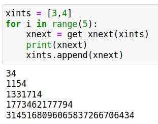
Although it must be clear by now, I am going to use the above terms to give the expression for L5:
So this is how a series expansion for √2 can be derived, of which the first four terms were given in the Sulbasutra expression! Note how each term is obtained recursively from the previous terms. It can be noted that the numbers become truly astronomical as each additional term is calculated!
In fact, looking at the expressions for L2, L3, etc., we can even obtain the final fraction that comes from adding up all the terms for L2, L3, etc. Suppose xn is the sequence [3, 4, 34, 1154, 1331714, . . . ], then L1 is given by:
Similarly, L2 is:
And similarly L3 is:
and so on. The above can also be converted into a computer script to return the corresponding numerator and denominator as follows:
import numpy as np
def get_final_fraction(n):
    assert n >= 0, "n must be greater than or equal to zero"
    # define initial sequence:
    xints = [3, 4, 34]
    # get the rest of the terms:
    for i in range(n):
        xnext = get_xnext(xints)
        xints.append(xnext)
    numerator = int(xints[-1]/2)
    xints.pop()    # remove the last term
    denominator = np.prod(np.array(xints)) # take the product of all the terms
    return int(numerator), int(denominator)
As an example, the output from my Jupyter Notebook of the fractional form from L1 is obtained as:

implying that the fractional form for L1 is 577/408. Similarly the fractional form for L2 is obtained as:

implying that
and similarly for L3:

which implies that
etc.
The Square Root Algorithm
In one of my previous posts I have talked about the so-called square-root algorithm, which goes like this:
1. Suppose the square root of N is needed.
2. Make an initial guess r1 for √N.
3. Find r2 = (1/2)(r1 + N/r2), which is the second iteration for √N.
4. Find r3 = (1/2)(r2 + N/r2), which is the third iteration for √N,
Etc., till the desired accuracy is achieved.
The algorithm works because if ri < √N, then N/ri > √N. Conversely, if ri > √N, then N/ri < √N. Hence √N always lies between ri and N/ri, and by successively taking the average of the two, r and N/r approach closer and closer with each iteration, i.e. r approaches √N.
What is fascinating is that if we use the above algorithm for finding the square root of 2 with 1+1/3 as the initial guess, i.e. the first two terms of the Sulba approximation, we get 1+1/3 + 1/(3×4) in the next iteration, i.e. the first three terms of the Sulba approximation. and which we have called L0 in this article. In the next iteration we get 1+1/3 + 1/(3×4) - 1/(3×4×34), i.e. the Sulba approximation itself, which we have called L1 in this article. And if we continue, we keep getting the next terms given by the sequence L2, L3, L4, etc. Thus, a knowledge of this algorithm in deriving the expression for the Sulba approximation by the authors of the Sulbsutras cannot be ruled out. It is also an interesting mathematical curiosity as to how the geometric method proposed by Datta and extended by Henderson produces the same results as the square root algorithm. This can indeed be proved using the relations developed above and will be done so in this article later.
Connection to the so-called Pell’s Equation
We have seen above how the sequence of fractions L0, L1, L2, L3, . . .etc. turn out to be more and more accurate approximations to √2. Consider any term in this sequence, say Li, and denote this by yi /xi, where both yi and xi are positive integers. Then:
(yi /xi)² ≈ 2,
i.e. yi² ≈ 2xi²,
i.e. yi² − 2xi² is a small integer not equal to zero. Let’s check out this difference for the first few cases. For L0, we have:
For L1, we have:
For L2, we have:
For L3, we have:
Thus, the cases examined above indicate that the rational approximations for √2 obtained from the Sulbasutra method have a remarkable property: the difference 2y²−x², where y is the numerator and x is the denominator, is always one! Thus x and y are integral solutions of the following equation
which is a special case of the so-called Pell’s equation. This latter is actually a family of equations given by
where N is a positive integer and integer solutions in x and y are sought. I am careful to call it the “so-called” Pell’s equation because although the equation is named after John Pell, an English mathematician from the 17th century, Hindu mathematicians Bhaskara II and Jayadeva had developed the chakravala algorithm by the 12th century and solved the above equation for several values of N centuries before it was solved in Europe. The case of N = 61 is especially difficult, and the solution for this was also given by Bhaskara II in the 12th century using the chakravala method. In 1657 Pierre de Fermat proposed the same problem to other mathematicians in Europe. As Andre Weil writes in his book Number Theory: An Approach Through History from Hammurapi to Legendre [4]:
His [Fermat’s] correspondence with Digby, and, through Digby, with the English mathematicians WALLIS and BROUCKNER occupies the next year and a half, from January 1657 to June 1658. It begins with a challenge to Wallis and Brouckner, but at the same time also to Frenicle, Schooten “and all others in Europe” to solve a few problems, with special emphasis upon what later became known (through a mistake of Euler’s) as “Pell’s equation”. What would have been Fermat’s astonishment if some missionary, just back from India, had told him that his problem had been successfully tackled there by native mathematicians almost six centuries earlier!
It has been noted by the historian of mathematics C. O. Selenius that [5]
[…] the chakravala method anticipated the European methods by more than a thousand years. But, as we have seen, no European performances in the whole field of algebra at a time much later than Bhaskara’s, nay nearly up to our times, equalled the marvellous complexity and ingenuity of chakravala.
Of course, since Hindu mathematical works were known in Europe through the Arabs and later through the Jesuits in Kerala, the question arises, to what extent was Fermat’s solution an “independent rediscovery”. Without going into it at the moment, what is relevant for the purposes of this article is that, as we have noted, the successive approximations for √2 obtained in this article using the Sulba method, i.e. L0, L1, L2, L3, . . . are such that, if we consider their fractional representation, their numerators and denominators are solutions of the so-called Pell’s equation Nx² + 1 = y² for the case N = 2. This can be proved by mathematical induction. I just share my rough hand written notes illustrating the basic idea in the following figure, where the the statement is proven for the special case of n = 4 assuming it to be true for n = 3. Generalizing it to arbitrary n is trivial.
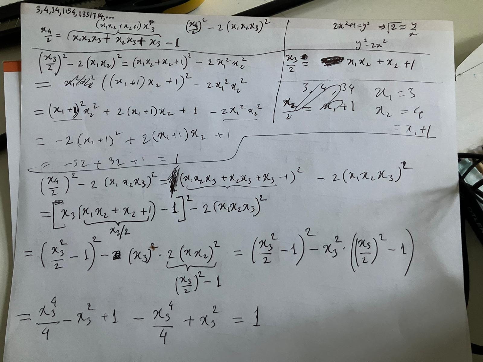
By the way, now that we have shown the above, a proof for why the Sulba method yields the same result as the square root algorithm is shown in the image below.
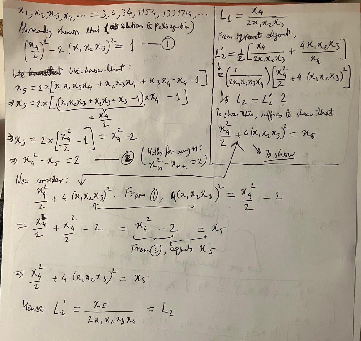
In the above, L1 is the usual sulba approximation discussed in this article; L2´ is the result from the square root algorithm at the next iteration using L1 as the initial guess, and L2 is the next approximation obtained using the Sulbasutra method and discussed in this article. The above image proves that L2 and L2´are equal. Generalizing it to arbitrary Ln and Ln´ is trivial.
On a personal note, I was initially flummoxed as to why the Sulbasutra method and the square root algorithm should give the same result because, after all, the two are entirely different methods and based on entirely different approaches. So I’m really happy that a long standing mystery has got cleared now!
Some Interesting Relations and a Simple Expression for the Series Expansion of √2
Based on the above observations, some interesting relations between the terms of the sequence x1, x2, x3, . . . can be found. For example, as we have shown above in the context of solutions to the so-called Pell’s equation, the following relation holds:
We have also shown in the context of the square root algorithm that
Combining the above two we get:
Or in general:
Another interesting relation that can be obtained is as follows. We have seen earlier that
Taking x4 common in the parenthesis, we get:
Noting that the term in the parenthesis equals x4/2, the above can be written as
Or, in general:
In other words, we have obtained a recursive relation between the terms xn and xn-1. (This relation has been mentioned by Henderson as well in his article.) This relation is really helpful in simplifying the form of the series expansion of √2. With the help of the above expression we can write:
Another interesting point to note is that solutions to the so-called Pell’s equation can serve as rational approximations to √N. If x and y are large integers which satisfy the solution, then √N can be approximated by the following rational form:
Indeed, this whole article is motivated by a closer examination of the square root of 2 and we have seen how the approximations L0, L1, L2, L3, . . . for the square root of 2 are solutions of the so-called Pell’s equation for N = 2. In fact, Brahmagupta, one of the early contributors to the chakravala method, gave examples for the purpose of demonstration for finding the square root of numbers by obtaining solutions to the appropriate equation [6].
Pell Numbers and Pell-Lucas Numbers
There were some other interesting facets that I stumbled across while learning more about the square root of two, which I would like to mention here for the sake of completeness. The square root of 2 is related to two sequences called the Pell numbers and the Pell-Lucas numbers. Both together form a sequence of rational approximations for the square root of 2 whose numerators and denominators satisfy the so-called Pell’s equation for N = 2. The Pell-Lucas numbers divided by 2 give the numerators and the Pell numbers give the denominators of the respective approximations. The Pell-Lucas numbers q(n) satisfy the following recurrence relation:
with q0 = q1 = 2.
The Pell numbers p(n) also satisfy the following relation:
but with p0 = 0 and p1 = 1.
Since the denominators and numerators of the successive approximations given by the Sulba method for the square root of two also satisfy the so-called Pell’s equation, they will also appear in the sequences. Here are two Python functions to generate these numbers along with their outputs:


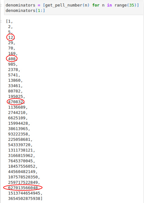
The terms corresponding to L0, L1, L2, L3, . . . are highlighted in the above images.
Summary
To summarize,
We derived a series expansion for the square root of 2 based on the method poposed by Datta and extended by Henderson, of which the Sulba approximation gives the first 4 terms.
The series is given by the following:
Writing out the first eight terms of the series:
We found also the fractional representations of the series:
We found the error between Ln² and 2. This is given by Ln² = 2 + wn-1². L1 is the approximation for the square root of two as stated in the Sulbasutras, and w0 = 1/(3×4×34), w1 = 1/(3×4×34×1154), etc.
We proved that the numerators and denominators of these fractions are solutions of the so-called Pell’s equation with N = 2.
We proved why the Sulba method gives equivalent results as the square-root algorithm and derived other recursive relations for the sequence x1, x2, x3, . . . .
The Pell numbers and Pell-Lucas numbers were introduced. The Sulba iterations, being solutions to the so-called Pell’s equation, also appear in these sequences.
References
[1] David W. Henderson. Square roots in the Sulba sutras, in Catherine A. Gorini (ed.) Geometry at Work: Papers in Applied Geometry, MAA Notes Number 53, Mathematical Association of America, Washington DC, 2000, 39–45.
[2] Thibaut, G. ‘On the Sulvasutras’. Journal of the Asiatic Society of Bengal, Vol. XLIV, (1875): pp. 227.
[3] Datta, Bibhutibhushan. The Science of the Sulba: A Study in Early Hindu Geometry. University of Calcutta, 1932.
[4] Weil, André. Number Theory: An Approach through History from Hammurapi to Legendre. Boston: Birkhäuser, 1984.
[5] Selenius, C. O. ‘Rationale of the Chakravala process of Jayadeva and Bhaskara II’. Historia Mathematica 2 (1975): pp. 167-184.
[6] (See here and here for the chakravala method in Hindu mathematics and Brahmagupta’s use thereof to obtain approximate square roots of non-square numbers such as 5. See here for understanding the mathematics behind the so-called Pell’s equation.)